Retrieval System

In Retrieval Augmented Generation (RAG) system, we often need to store some documents which probably contains some specific knowledge or information that LLM agents can use as context to reply the user’s question. The examplel documents can be CSV files, PDF files, etc. To make this work end to end, we need to first store the documents in a database or search engine, then the agent can retrieve the information when needed.

In this post, we will talk about

1. write path
2. read path
3. vector search

Write Path

Let’s use PDF as an example here. A PDF file page can contain multiple forms of information, for example, text, table, image, charts, etc. To have better retrieval performance, each form should be parsed and chunked well.

Parsing

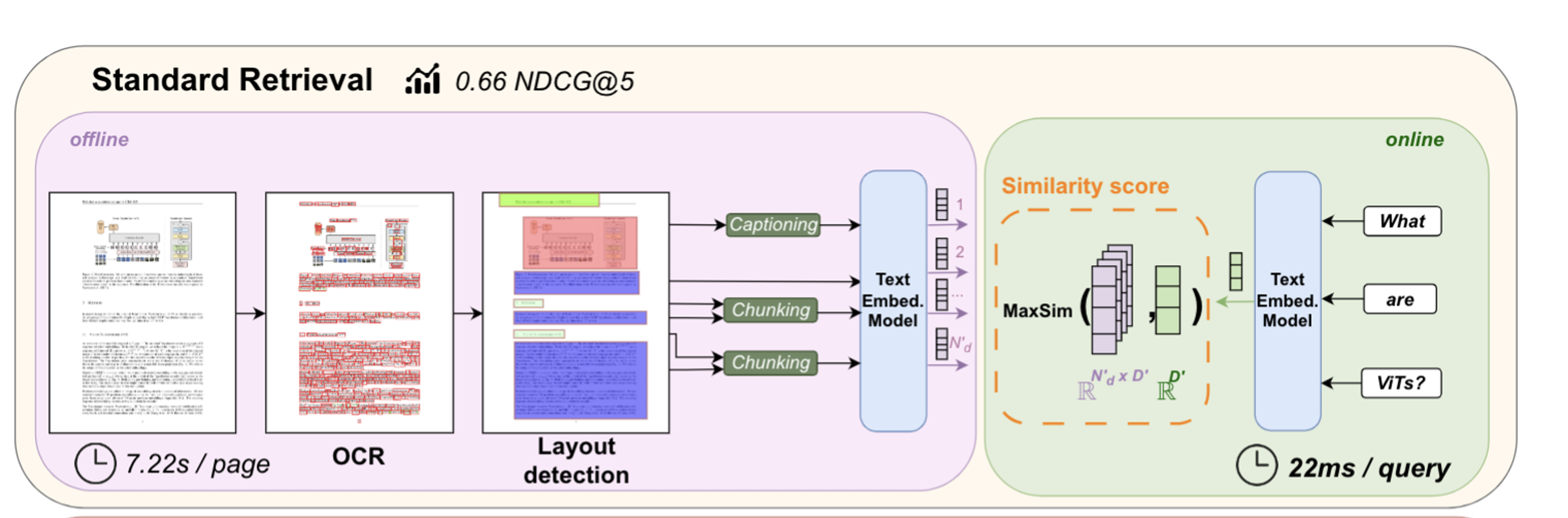
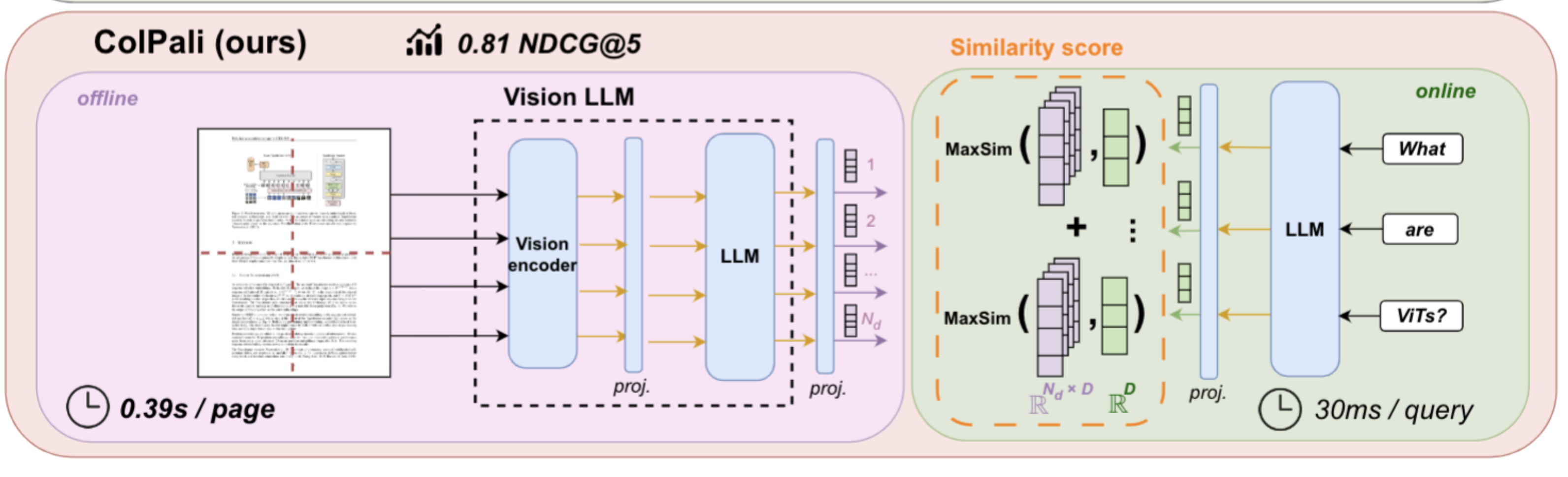
What problem does parsing a PDF file solve? You have a file, but to store it in a database so that an LLM agent can use, we need to convert the file into texts or/and images. The most common way to parse a PDF file is to use Optical Character Recognition (OCR) to convert the PDF file into texts. This works well for text-based PDF files. But for visual-rich information types liketables, images, charts, etc, the OCR parsing performance is not good. This is not surprising because a table is a 2D structure, and OCR is a 1D structure. The diagram below illustrates the standard OCR parsing and chunking process from ColPali paper[1]

Improve visual-rich information parsing

As Visian Language Model (VLM) has been getting better and better, we can use VLM to parse the visual-rich information types like tables, images, charts, etc. Just iterate the prompt.

Chunking

Why chunking? I think a few reasons:

1. The context window of LLM is limited. You don’t want to feed the whole document to the LLM because the generation quality might be low.
2. Even if the context length is larger and larger for SoTA models, feeding LLM with too much information might not be a good idea[2].

After parsing, we have a long sequence of characters. We need to divide them into smaller chunks before storing them in the database. Some ways to do this are:

1. Sliding window chunking: just pre-define a window size and slide it through the text.
   • Pros: simple and fast
   • Cons: the boundary of the chunks might be awkward
2. Semantic chunking: use LLM to divide the text into semantic chunks.
   • Pros: the chunks are more natural
   • Cons: the cost is higher

Skip parsing and chunking

This is the idea from ColPali paper[1]. Instead of parsing and chunking the PDF file, we can use text-aligned embedding model(CLIP[3]) to directly embed each PDF page. From their experiments, the performance is better than the standard OCR parsing and chunking, especially for visual-rich information types.

Pros:

• No need to think about the chunking strategy
• The visiual information can be well preserved if you have a good text-aligned embedding model

Cons:

• The pure text embedding model cannot be used
• For the visual information that spans multiple pages, the retrieval performance is not good

Embedding

The chunks will be used by LLM agent to generate response to the user’s question. So ideally the agent should find the most relevant chunks to the user’s question. This finding process is a search process. To better search, we need to have a good representation of the chunks. And usually the representation is a embedding vector. We will talk more about vector search in this post. There are many models that can be used for this purpose. Some of them are pure-text models like DRAMA[4] and some of them are text-aligned embedding models like CLIP[3].

Note that the performance of the retrieval is highly dependent on the quality of the embedding model. It is a good idea to do some ablation study on different models.

Search engine, vector database

Now we have chunks, and we have embedding model to create the dense vector for each chunk. We need to store the embedding together with the original chunk in a vector database. FAISS can be used to cluster the dense vectors for efficient similarity search.

Read Path

Now we have successfully stored the chunks and their embeddings in a vector database. Embeddings will be used for the similarity search and original chunks will be used for the response generation. That is great! Let’s imagine, we have a user query, what is the total revenue of the company in 2024? If your chatbot doesn’t know the answer, it will search the vector database for the most relevant chunks and use them as context to generate the response.

Query rewrite

Sometimes, the user query is not very specific or the chat history is needed as the context of the question, we probably need to rewrite the query a little bit before using it to search the vector database. For example, in the chat history, the user is asking about a product, and then user asks How much? we need to augment the query with the product name.

Embedding

To do efficient similarity search, we need to generate embedding for the query. Obviously this embedding model should be the same as the one used for the chunk embedding.

Hybrid search

Sometimes, pure embedding search might not work well. For example, for each chunk embedding, there might be different versions. We need to specify the version of the chunk embedding to retrieve the correct chunk. To do this, we can use hybrid search. It is nothing but term-based search and vector search. Term here is a term used in the inverted index of the search engine. A document contains many keywords, the document -> list of keywords is a forward index. And the keyword -> list of documents is an inverted index. Inverted index can help efficiently find the documents that contain the query terms. In our example above, the term is the version id.

Vector search

Before wrapping up, I want to talk a little bit about the vector search. Because I find this is a really interesting topic. The problem setup is we have a query, and we want to find the top k most relevant chunks from the vector database which is also called k-nearest neighbor search. Many discussion here is referencing FAISS

Naive search

Given a query embedding, we will go through every candidate in the database, compute the distance metric between them, and return the top k candidate as the results.

The shortcoming is obvious. When the number of candidates in the database is really large, this speed of returning results would be very slow. To improve this, approximate K nearest neighborhood(ANN) search is invented. The trade-off is speed vs recall. The speed is improved but the true k nearest neighbor might not be returned. The recall is number of true k nearest neighbor returned / k.

IVF

IVF is inverted File. The number of centroids/clusters is nList. For example IVF_64. The candidates in the database will be preprocessed by clustering them into groups. The number of clusters is a hyperameter. Each cluster has its own centroid which will be used in the search. nProbs is another hyperameter.

So in search,

1. the nProb nearest centroids to the query will be found first
2. Then look at the candidates belong to those clusters and find the K nearest candidates to the query as the returned results

You can see that the speed will be improved compared to Exact KNN. But the recall would hurt.

HNSW: Hierarchical Navigable Small World[5]

This is another ANN algorithm/data structure. The graph is a multi-layer graph. The top layer will have fewest number of node(one datapoint in the database) while the lowest layer will have ALL nodes. On each layer, each node is bi-directionally connected to a few number of neighbors. During search of the K nearest neighbor to a query, the search will start at the top layer with an entry point. For each layer, efSearch number of candidates will be returned as the search results. They will also be served as the entry points in the next layer. Finally at the bottom layer, the K nearest neighbor will be returned which are in the search results of the bottom layer.

Search on each layer

Before talking about the graph construction(write) and search(read), let’s first talk about the search algorithm on each layer because it will be used in both construction and search.

The input of the search on each layer

1. the query embedding
2. the entry points of this layer
3. ef: expansion factor, for construction it is efConstruction, for search it is efSearch. This is the number of candidates returned on each layer

The search will start from the entry points. Search the neighbors of the closest candidate. Update the candidate set and the returned set. The termination criteria is that the current closest candidate is further to the query than the furthest element in returned set.

Search-Layer algorithm

Algorithm 2  SEARCH-LAYER(q, ep, ef, lc) 
Input: query element q, enter points ep, number of nearest to q elements to return ef, layer number lc

Output: ef closest neighbors to q 

1 v ← ep // set of visited elements 

2 C ← ep // set of candidates 

3 W ← ep // dynamic list of found nearest neighbors 

4 while │C│ > 0  

5 c ← extract nearest element from C to q, search the neighbors of it and remove c from C

6 f ← get furthest element from W to q 

7 if distance(c, q) > distance(f, q)  
     8 break // all elements in W are evaluated 

9 for each e ∈ neighbourhood(c) at layer lc // update C and W 
   10 if e not visited: 
          11 v ← v ⋃ e 
      
          12 f ← get furthest element from W to q  
          
          13 if distance(e, q) < distance(f, q) or │W│ < ef 
              14 C ← C ⋃ e 
              15 W ← W ⋃ e 
              16 if │W│ > ef  
                   17 remove furthest element from W to q 18 return W
18 Return W

Select Neighbors Simple

Input:

1. Given a pool of candidates for neighbors
2. number of neighbors, M
3. query

Just go through each candidate and find the M closest candidates as the neighbors. Select neighbors with heuristic Only add to the returned list(neighbors) when the distance between this element is closer to query than any other existing ones in the returned list

Construction of graph

The goal of the construction is to construct the neighborhood links between each inserted datapoint and the existing datapoints in the database. The neighbors here means the closest nodes to the inserted datapoints on each layer. Because those neighbors will be used in Search as you can see above in the search layer algorithm.

Inputs

1. The expansion factor efConstruction
2. The number of neighbors for each node, M
3. Maximum number of neighbors for each node, M_max
4. level/layer generation parameter m_l
5. query

Algorithm

1. identify the starting layer: this datapoint will be inserted to this layer and all layer below it, with the help of m_l
2. When the layer is above the current top layer, set the hnsw graph entry point as query
3. Identify the entry point of the layer. It will start from the top layer and search each layer with ef = 1, only returning one closest candidate on each layer until the starting layer.
4. For each layer starting from the layer identified in 1,
   1. search this layer to find the efConstruction candidates with search layer algorithm.
   2. find the neighbors from the candidates above with the select neighbor algorithm above, total number is M
   3. Add bidirectional link between query and neighbors
   4. Prune neighbors of neighbor list in 3.
   5. Since we add bidirectional link in step3, for some neighbors, their own neighbors might exceed the M_max
   6. The prune will just use the neighbor select algorithm above and the candidates are all neighbors if the number of them exceeds M_max

Search

This is where the k-nearest neighbor happens

Input

1. The hnsw graph
2. The query
3. efSearch
4. k: how many results to return

Algorithm

1. starting from the entry point of hnsw
2. search_layer with ef=1 for layer L to layer 1
3. for layer 0, search_layer with ef=efSearch
4. select K nearest in the results list from 3

So to summarize, the idea is find the one closest node for layer L to layer 1 by traversing the neighbors until stop criteria and then go to next level do the same thing. For layer 0, the candidate pool is expanded so more exploration in layer0.

Reference

[1] @misc{faysse2025colpaliefficientdocumentretrieval, title={ColPali: Efficient Document Retrieval with Vision Language Models}, author={Manuel Faysse and Hugues Sibille and Tony Wu and Bilel Omrani and Gautier Viaud and Céline Hudelot and Pierre Colombo}, year={2025}, eprint={2407.01449}, archivePrefix={arXiv}, primaryClass={cs.IR}, url={https://arxiv.org/abs/2407.01449}, }

[2] https://research.trychroma.com/context-rot

[3] @misc{radford2021learningtransferablevisualmodels, title={Learning Transferable Visual Models From Natural Language Supervision}, author={Alec Radford and Jong Wook Kim and Chris Hallacy and Aditya Ramesh and Gabriel Goh and Sandhini Agarwal and Girish Sastry and Amanda Askell and Pamela Mishkin and Jack Clark and Gretchen Krueger and Ilya Sutskever}, year={2021}, eprint={2103.00020}, archivePrefix={arXiv}, primaryClass={cs.CV}, url={https://arxiv.org/abs/2103.00020}, }

[4] https://arxiv.org/pdf/2502.18460

[5] @misc{malkov2018efficientrobustapproximatenearest, title={Efficient and robust approximate nearest neighbor search using Hierarchical Navigable Small World graphs}, author={Yu. A. Malkov and D. A. Yashunin}, year={2018}, eprint={1603.09320}, archivePrefix={arXiv}, primaryClass={cs.DS}, url={https://arxiv.org/abs/1603.09320}, }