nano-vllm is one of my favorite projects in 2025. It only has ~1200 lines of Python code. I learned a lot from it. Highly recommend folks who are interested in LLM inference optimization to check it out!
From nano-vllm we can see that inference optimization can be categorized into two aspects:
- System optimization
- Paged Attention
- Batching
- Scheduler
- Model optimization
- Tensor parallel
- Kernel fusion
- Weight packing
Tensor parallel(TP) is one of the key techniques which not only can speed up inference by doing the compute across multiple GPUs and each GPU only needs to load a part of the model weights but also can improve the overall throughput by batching more input tokens since the KV cache is also distributed across multiple GPUs.
In this blog, I am going to use Qwen3 0.6B dense model architectureas an example to illustrate TP.
Model Architecture
The dense Qwen3 0.6B is a typical transformer model. It starts with an embedding layer, then 28 layers of transformer blocks, and finally an LM head to project the hidden states to vocabulary space. We will follow this order to illustrate TP.
TP for Embedding Layer
The embedding layer is nothing but a big matrix with shape [vocab_size, embedding_dim], where vocab_size is the number of unique tokens in the vocabulary and embedding_dim is the dimension of the embedding vectors. With TP, when loading this big matrix, it will be split into multiple parts and each part will be loaded into a different GPU. The question is how to split? The answer is that the split is done along the vocab_size dimension.
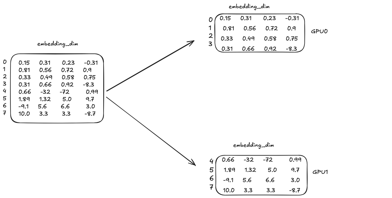
In the above example, the vocab size is 8 and embedding dimension is 4. And we have 2 GPUs. The first GPU will load the first 4 rows of the matrix and the second GPU will load the last 4 rows of the matrix. Let’s use a concrete example input to illustrate how the TP works in embedding layer. Let’s say the input is 3 tokens with ids [0, 4, 3]. The embedding matrix can be seen as a lookup table for the input token ids. For example, for token id 0, we will use the first row.
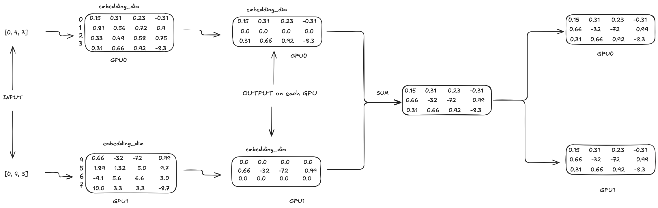
Each GPU will have the same input [0, 4, 3]. For GPU0, since the range of token ids is [0, 3]. So for second token id 4, its output will be all 0s on GPU0. Similary, for GPU1, the range of token ids is [4, 7]. So for first token id 0 and third token id 3, its output will be all 0s on GPU1. The most intersting part is how to sync the output of each GPU to get the final output. In this case, we can simply add the output of each GPU together to get the final output. And then the final output will be synced back to each GPU as the input for the next layer. In PyTorch, this sync operation is achieved by all_reduce.
TP for Transformer Block
Each transformer block has 2 sub-layers: attention and MLP.
TP for Attention
The attention operation is as follows: \(\text{Attention}(Q, K, V) = \text{softmax}(\frac{QK^T}{\sqrt{head\_dim}})V\)
And $Q = X W_q^T$, $K = X W_k^T$, $V = X W_v^T$, where $X$ is the input to the attention layer, $W_q$, $W_k$ and $W_v$ are the weight matrices for query, key and value respectively.
And there is also an output projection operated on the attention output.
\[O = \text{Attention}(Q, K, V) W_o^T\]So we can see that there are 4 weight matrices involved in the attention layer. With TP, we need to split each of them and load each split into different GPUs.
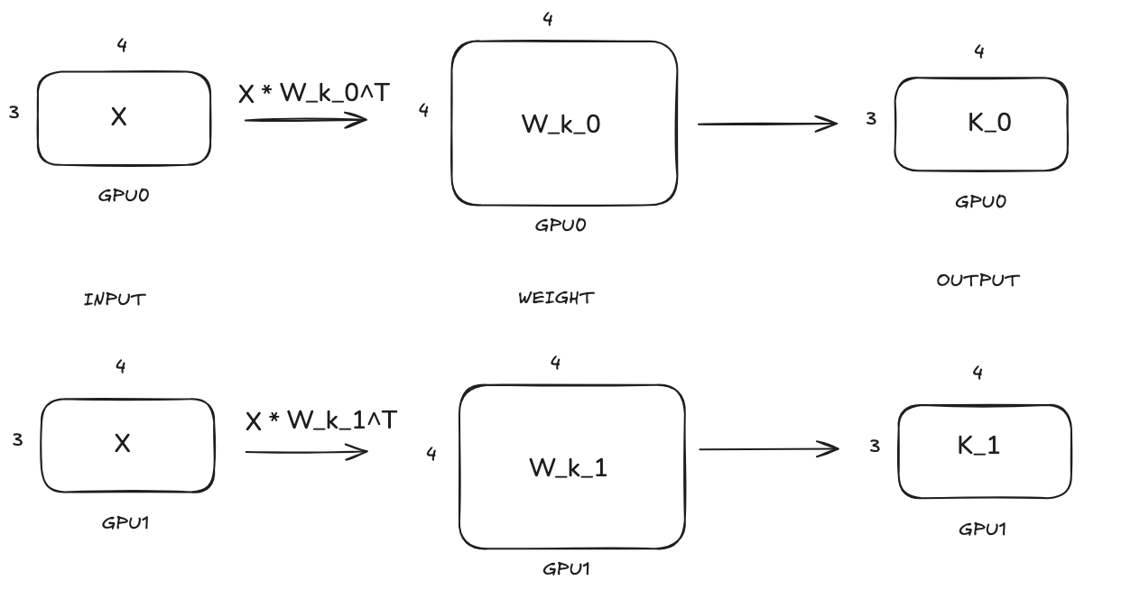
Still use the same example. The input of attention layer X is of shape [3, 4]. And let’s say query, key and value each has 2 heads and head dimension is 4. So the shape of W_q, W_k and W_v are [8, 4], [8, 4] and [8, 4] respectively. So the question is how to divide them into different GPUs? We will divide them along the row dimension. We will explain why we do this later.
Query:

Key:
Value:

We can see that query, key and value projections follow the same TP computation pattern that the weight matrices are split along the row dimension and each GPU will hold part of the projection results.
The attention operation on each GPU will be as follows:
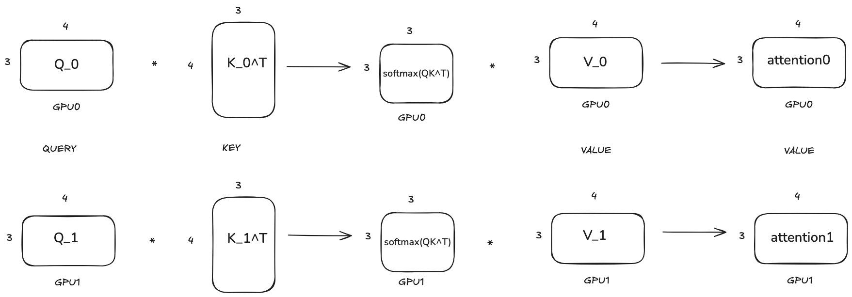
We can see that by splitting along the row dimension of the weight matrices of query, key and value, the attention operation can be done on each GPU separately and there is no need to communicate between GPUs during the whole attention operation which is awesome!
And finally, we need to do the output linear projection on each GPU. Since we need to change the output dimension back to embedding_dim, the shape of the weight matrix W_o will be [4, 8]. So we need to split along the column dimension this time.
Before going to the MLP layer, the output of the attention layer output needs to be synced with sum and can be achieved by all_reduce in PyTorch.
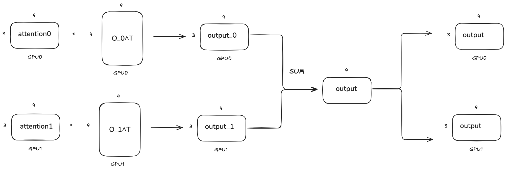
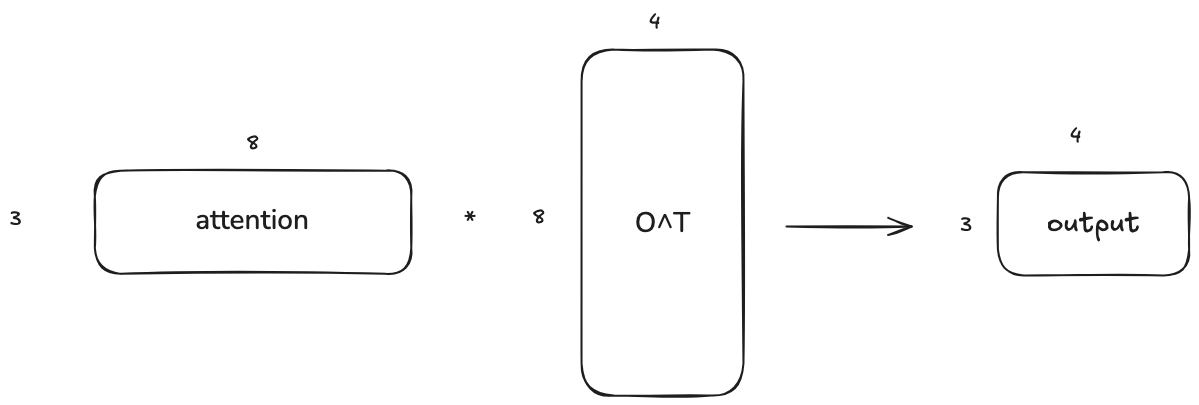
I just want to talk a little bit more about why the sync is achieved by summing up the output matrices element-wise. The output projection of attention layer is nothing but a matrix multiplication. The left is the output of the attention operation and the right is the weight matrix. If we only have 1 GPU, the it will look like this:
Since the matrix multiplication can also be done in a block-wise manner, it can also be visualized as follows when we divide each matrix into 2 blocks:
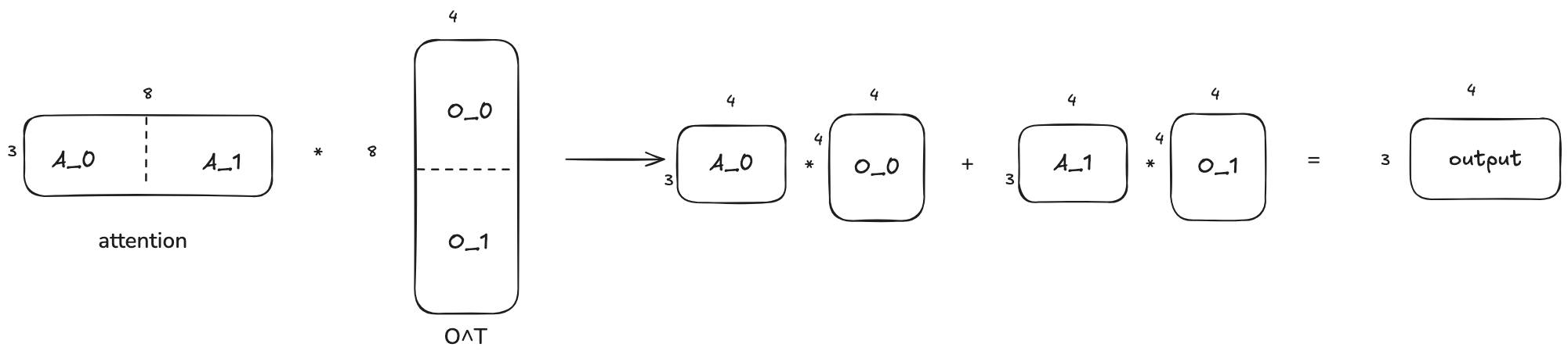
And for 2 GPUs, A_0 is the attention output on GPU0 and A_1 is the attention output on GPU1. And O_0 is the weight matrix on GPU0 and O_1 is the weight matrix on GPU1. So the final output is the sum of the output of each GPU.
TP for MLP
For dense Transformer model, the MLP layer is very simple. It has two linear projections. The first linear projection is from embedding_dim to intermediate_dim and the second linear projection is from intermediate_dim to embedding_dim.
Where $X$ is the input to the MLP layer, $W_1$ and $W_2$ are the weight matrices for the first and second linear projections respectively.
And with TP, we need to split each of them and load each split into different GPUs. And the computation pattern is very similar to the attention layer. You can see the first matrix multiplication the same as Q projection where the weight matrix is split along the row dimension and the second matrix multiplication the same as O projection where the weight matrix is split along the column dimension. So I will not go into the details here.
TP for LM Head
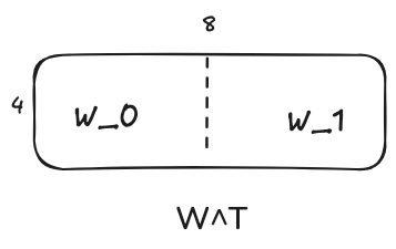
LM head is projecting the hidden states to vocabulary space. Its weight matrix is of shape [vocab_size, embedding_dim] which is the same as the embedding matrix. And that is why some models make those 2 matrices the same. And same as the embedding matrix, this matrix is split along the row dimension(vocab_size dimension). We will use W denote this matrix and X as the input. The linear projection works like
The transpose of W is split as follows
And the computation on each GPU will be as follows:
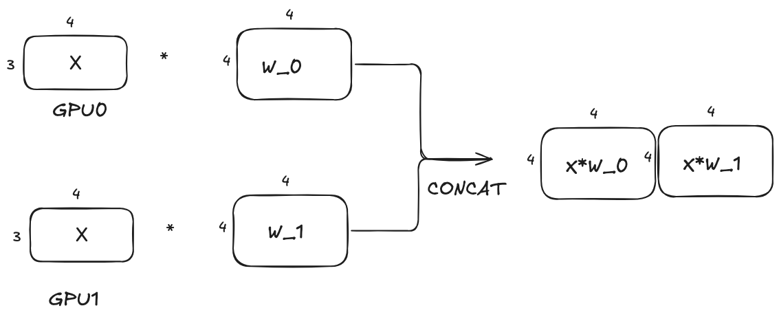
We can see that the sync is achieved by concatenating the output of each GPU along the column dimension of the outputs. This is also due to the block-wise matrix multiplication. In PyTorch, this sync operation is achieved by
- gather: if you want one GPU to get the final output.
- all_gather: if you want all GPUs to get the final output.
Final remarks
I find TP as a very creative way to make inference with very large model possible. In this blog, we are using a dense model as an example. For Mixture of Experts(MoE) model, the MLP part in each transformer block actually has multiple MLP layers. Expert Parallel can be used to distribute the MLP layers across multiple GPUs. I may talk about it in the future.