This blog is a companion blog to my nanoquantization repository. While there are many excellent blogs providing high-level overviews of AWQ and other quantization algorithms(nvidia blog), I found that the fascinating implementation details are often glossed over. In this blog, I want to dive deep into the nitty-gritty implementation details that I found really, really interesting and want to share with my readers.

What is quantization and why

In terms of Machine Learning models, quantization is a process to compress the model weights so that the total size of the model can be reduced significantly. For example, Qwen3 model is using bfloat16 during training which means each model weight is 16 bits floating point number. If we can compress the model weight to 4-bit, then its size will be reduced to 1/4 of the original size. This is a significant reduction and can be very helpful for the deployment of the model.

How?

As mentioned above, quantization will convert a floating point number to a lower precision integer. For example, AWQ uses 4-bit quantization to compress the model weights. How does it work? The quantization formula is very simple

\[q = \text{round}(w / S)\]

where $w$ is the floating point number, $S$ is the scale factor, and $q$ is the quantized value.

Let’s use a concrete example to illustrate this.

\[W = \begin{bmatrix} 0.2 & -1.6 & 2.9 \\ -0.1 & 0.5 & -0.8 \\ 1.2 & -2.3 & 0.7 \end{bmatrix}\]

If we quantize this weight matrix row by row, then for each row, it will have its own scale factor. And if the target quantization precision is 4-bit, we can calculate the scale factor for each row as follows:

\[S_1 = \frac{\max(abs(W_1))}{7} = \frac{2.9}{7} = 0.4\] \[S_2 = \frac{\max(abs(W_2))}{7} = \frac{0.8}{7} = 0.1\] \[S_3 = \frac{\max(abs(W_3))}{7} = \frac{2.3}{7} = 0.3\]

where 7 is the maximum value that can be represented by a signed 4-bit integer (range: -8 to 7).

Then we can quantize the weight matrix row by row as follows:

\[Q_1 = \text{round}(W_1 / S_1) = \text{round}(\begin{bmatrix} 0.2 & -1.6 & 2.9 \end{bmatrix} / 0.4) = \begin{bmatrix} 1 & -4 & 7 \end{bmatrix}\] \[Q_2 = \text{round}(W_2 / S_2) = \text{round}(\begin{bmatrix} -0.1 & 0.5 & -0.8 \end{bmatrix} / 0.1) = \begin{bmatrix} -1 & 5 & -8 \end{bmatrix}\] \[Q_3 = \text{round}(W_3 / S_3) = \text{round}(\begin{bmatrix} 1.2 & -2.3 & 0.7 \end{bmatrix} / 0.3) = \begin{bmatrix} 4 & -8 & 2 \end{bmatrix}\]

where round is the rounding function to the nearest integer.

How to convert back to floating point or de-quantize?

The de-quantization process is very simple. We can use the following formula:

\[w = q * S\]

where $q$ is the quantized value, $S$ is the scale factor, and $w$ is the floating point number.

Let’s use the same example to illustrate this.

\[W_1 = Q_1 * S_1 = \begin{bmatrix} 1 & -4 & 7 \end{bmatrix} * 0.4 = \begin{bmatrix} 0.4 & -1.6 & 2.8 \end{bmatrix}\] \[W_2 = Q_2 * S_2 = \begin{bmatrix} -1 & 5 & -8 \end{bmatrix} * 0.1 = \begin{bmatrix} -0.1 & 0.5 & -0.8 \end{bmatrix}\] \[W_3 = Q_3 * S_3 = \begin{bmatrix} 4 & -8 & 2 \end{bmatrix} * 0.3 = \begin{bmatrix} 1.2 & -2.4 & 0.6 \end{bmatrix}\]

As we can see, the de-quantized values are very close to the original values. But there is still some difference which leads to the quantization error. Quantization error is the cost that we need to pay for the compression. And many quantization algorithms aim to minimize it.

Post Training Quantization(PTQ)

There are different ways to quantize the model weights. Post training quantization is just taking the trained model weights and quantize them without any training or fine-tuning involved. The benefit is that you can get the quantized model very quickly. And the downside is that the quantized model may not be as performant as the approach that invovles quantization in training or fine-tuning.

Quantization aware training is a popoular way to quantize the model weights during training. As it is not the focus on this blog, readers can refer to this nvidia blog and unsloth blog for more details.

Round to nearest(RTN)

RTN is a very simple PTQ approach which will do nothing but taking the model weight and quantize them to the nearest integer with the formula mentioned above. Compared to other more advanced and more complicated PTQ approaches, RTN is much simpler and faster. But the performance of the quantized model is not as good as the more advanced approaches, for example AWQ.

RTN works well for 8-bit quantization but not that good for lower bit.

Activation Aware Weight Quantization(AWQ) for 4-bit quantization

The key insight from the paper is that not all model weights are equally important. Some weights are more important than others. And this importance is measured by the magnitude of the corresponding activation. The larger the magnitude of the activation, the more important the corresponding weight is. Let me use a quick example to illustrate this.

Activation or input to a lienar layer is as follows: \(X = \begin{bmatrix} 1.0 & 2.0 & 3.0 \\ 4.0 & 5.0 & 6.0 \\ 7.0 & 8.0 & 9.0 \end{bmatrix}\)

The weight matrix is as follows: \(W = \begin{bmatrix} 0.2 & -1.6 & 2.9 \\ -0.1 & 0.5 & -0.8 \\ 1.2 & -2.3 & 0.7 \end{bmatrix}\)

Then the output of the linear layer is as follows: \(O = X W^T\)

If we take a look at the input column by column, and get the average absolute value for each column, we will get the following: \(\text{avg}(abs(X)) = \begin{bmatrix} 4.0 & 5.0 & 6.0 \end{bmatrix}\)

This absolute value will be used to measure the importance of the corresponding weight. The larger the absolute value, the more important the corresponding weight is.

This is why AWQ needs a calibration dataset because it needs to find the important weight based on the activation of the calibration dataset.

Upscale the important weight

The proposed approach is to NOT quantize the important weight to keep their precision. But in reality, it is hard to store floating point weight and integer weight in the same tensor. So what they do is to upscale the important weight to improve the precision after quantization. I will call this upscale factor as $scale\_important\_weight$. It works as follows:

\[final\_quantized\_weight = quantize(float\_weight * scale\_important\_weight) / scale\_important\_weight\]

Let’s use a simple example to illustrate why this helps preserve the precision for more important weight.

The Setup:

• Original Weight (w): 0.65

Case 1: Standard Quantization

We simply round the weight to the nearest step.

\[w_{quant} = \text{round}(0.65) = 1.0\] \[\text{Error} = |1.0 - 0.65| = \textbf{0.35}\]

Case 2: AWQ Scaling (Scale Factor s = 2)

In AWQ, we multiply the weight by s = 2 before quantizing.

1. Scale Up: \(w' = 0.65 \times 2 = 1.3\)

2. Quantize (using the same Δ = 1): \(w'_{quant} = \text{round}(1.3) = 1.0\)

(Note: It maps to integer 1, but this “1” represents a value in the scaled space)

3. De-scale (The Equivalent Effect):

Since we multiplied w by 2, and we divide the activation x by 2 later, the effective weight the network “sees” is the quantized value divided by 2.

\[w_{effective} = 1.0 / 2 = \textbf{0.5}\] \[\text{Error} = |0.5 - 0.65| = \textbf{0.15}\]

Result:

• Standard Error: 0.35
• Scaled Error: 0.15

Weight Packing

The target precision for AWQ is 4-bit. And every 8 4-bit quantized weights will be packed into a 32-bit integer for effient data transfer between GPU memory(HBM) and GPU registers. Let’s say we have 8 4-bit quantized weights and packed in a naive way as follows

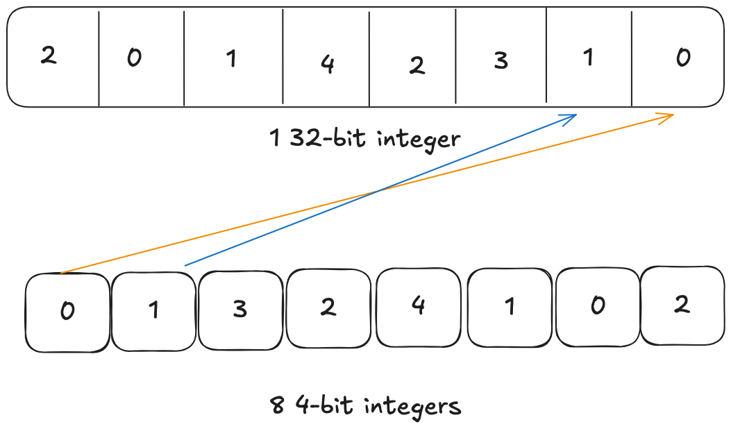
We can see that the first weight is placed at the lowest 4 bits and second weight is placed at the next 4 bits and so on. When GPU loads the 32-bit data from HBM, it will read the 32-bit integer into a 32-bit register. Remember that our target data type that we want to do the computation is 16-bit float or bfloat16. So the GPU needs to unpack this 32-bit integer into 8 16-bit floats which is 4 32-bit registers. If we use this naive packing, to unpack the first pair of 4-bit weights (0 and 1), the assembly instructions will be as follows:

We need to get Element 0 into the bottom half (bits 0-15) and Element 1 into the top half (bits 16-31) of the output register.

Unpacking Pair 1 (Elements 0 & 1)

1. COPY Input to Temp - Copy the input register to a temporary register
2. AND Temp, 0xF → Temp now holds Element 0 in the bottom
3. SHR (Shift Right) Input, 4 → Moves Element 1 to the bottom (bit 0)
4. AND Input, 0xF → Clears garbage bits
5. SHL (Shift Left) Input, 16 → Moves Element 1 to the top (bit 16)
6. OR Temp, Input → Combines them (Result: Int16x2)
7. CVT (Convert) Int16x2 to BF16x2 - Convert to bfloat16
8. MUL (Multiply) Scale - Multiply by the scale factor

Instruction Count: 8 instructions for this pair.

But modern GPU has capability to be more efficient. It can manipulate the high 16-bit and low 16-bit of the 32-bit integer in a single instruction. So if we pack the 8 4-bit integers smarter, we can utilize this vectorized instructions to speed up the unpacking process. How about packing like this

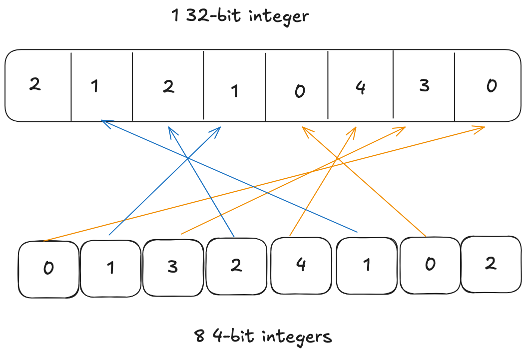
We place the first weight at lowest 4-bit and second weight at bits between 16 and 20. Now because first and second weights are in lower 16-bit and higher 16-bit respectively, one instruction can work on both of them at the same time.

Unpacking Pair 1 (Elements 0 & 1) Element 0 is already at Bit 0, and Element 1 is already at Bit 16.

1. AND Input, 0x000F000F → Cleans both values instantly. (Result: Int16x2)
2. CVT (Convert) Int16x2 to BF16x2 - Convert to bfloat16
3. MUL (Multiply) Scale - Multiply by the scale factor

Instruction Count: 3 Instructions for this pair(we reduce the instruction count from 8 to 3 -> faster unpacking)

I hope this illustration can help understand why AWQ uses this weird packing order.

Whole workflow

I expand on some details of AWQ that I find very very intersting above. For this section let’s get some sense about the whole workflow of it.

1. A small calibration dataset is used to get the magnitude of the activation(input) for each linear layer
2. The activation magnitude will be used to scale the corresponding weight so that weight with larger activation will be scaled up to minimize the quantization loss.
3. Remember in section Upscale the important weight, this scale will also be used to divide the quantized weight. This division actually happens at the previous layer of each quantized layer. For example, RMSNorm layer is the previous layer of q_proj, k_proj, v_proj in the attention layer. RMSNorm layer weight will be divided by the scale factor.(NOTE: this scale factor is NOT the scale factor when doing the quantization in the math formula in section How?, it is AWQ specific scale factor to upscale the important weight)
4. After the weights have been adjusted by the activation magnitude, then those weights will be quantized in the way mentioned in section How?. And the scale factors to do the quantization will be stored in the quantized model for de-quantization later.
5. Every 8 quantized 4-bit weights will be packed into a 32-bit integer smartly and weirdly.
6. During dequantization, the weight unpacking will be done to get the bfloat16 or float16 depending on the data type during training.
7. Then the dequantized weights will be used to do the matrix multiplication with their inputs.

NOTE: to be more efficient, step 6 and step 7 can be fused into a single kernel. If you are interested in the details, please take a look at the nanoquantization triton kernel which is derived from AutoAWQ with my comments.