Problem Statement
GPU memory is precious and limited. For optimizer like Adam[1] or AdamW[2], the memory usage is about 2x of the model parameters. This is because for each parameter, we need to store the first and second moment of its gradient during the training process. So for example, if a model has 1B parameters, and the data type of a parameter is 32-bit float, then the memory usage for the model parameter is 1B * 4 bytes = 4GB. And for the optimizer, the memory usage is 2 * 4GB = 8GB. This is of course a lot.
So the question is if the memory usage of the optimizer can be reduced while not sacrificing the model performance? The answer is yes. In this blog, I will mainly talk about a paper 8-bit Optimizers via Block-wise Quantization [3].
My Experiment
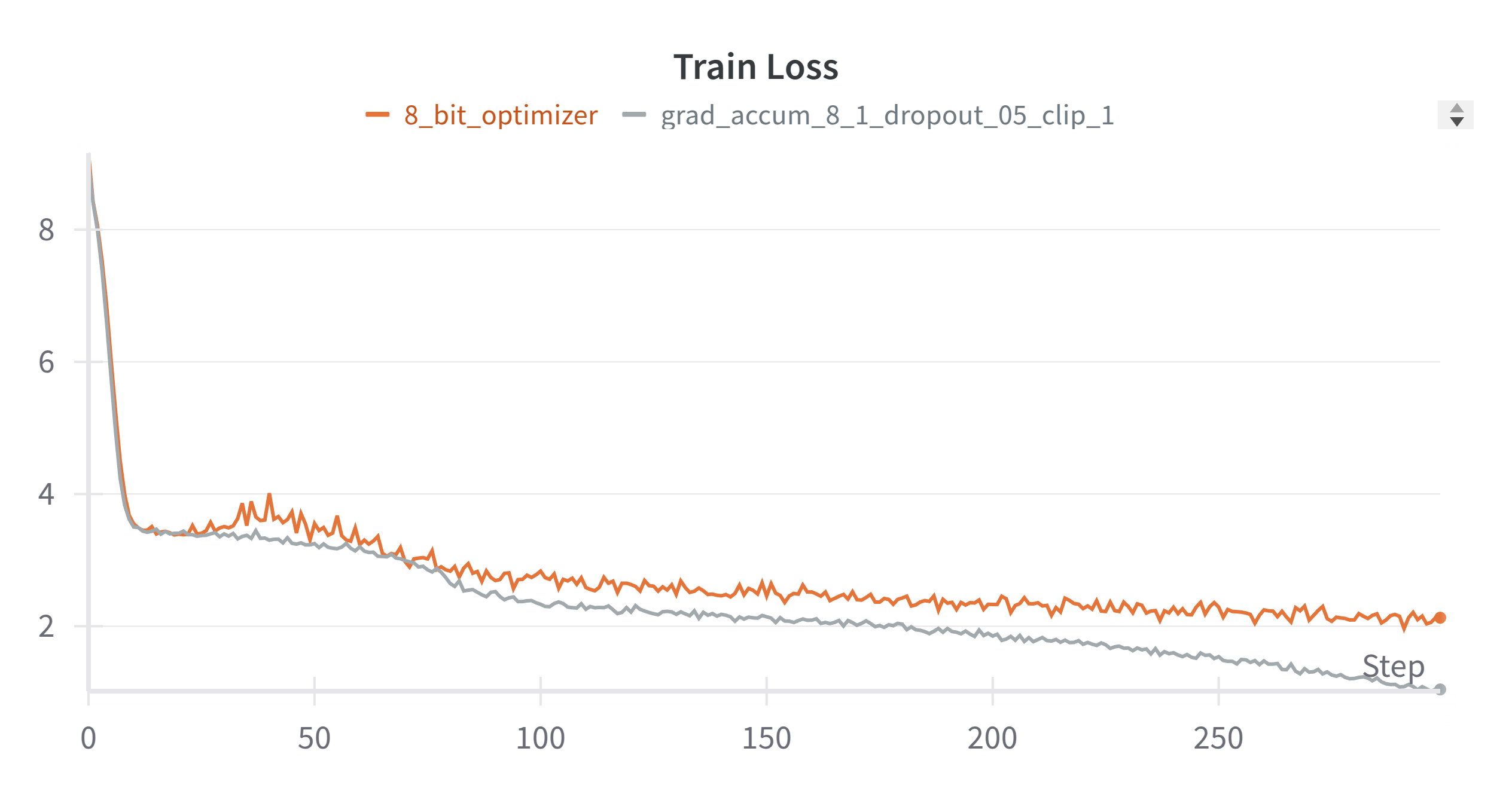
I tried the 8-bit AdamW optimizer on my nano DeepSeekV2 project(WIP). It reduced the memory usage from 24GB to 19GB which is a lottt. And the training loss seems good although the convergence is slower than the 32-bit optimizer.
Quantization
The reason that why the optimizer states use 2x memory of the model parameters is because it uses the same data type as the model parameters which is often 32-bit float or 16-bit float(bfloat). If the data size can be 8-bit, then the memory usage can be reduced to $\frac{1}{4}$ or $\frac{1}{2}$ of the model parameters. That is great, right? The process converting the 32-bit float or 16-bit float to 8-bit is called quantization.
What is quantization and how does it work? To simplify the problem, let’s consider the case of 2-bit quantization. We have a pool of quantization candidates. For 2-bit quantization, there are 4 candidates. Let’s say they are $-1.0, -0.5, 0.5, 1.0$. And the model parameters are $-5.5, -2.5, 0.5, 3.5$. The quantization process works as follows:
Step 1: Find the largest absolute value of the model parameters. In this case, it is $5.5$.
Step 2: Divide the model parameters by the largest absolute value. So the model parameters become $-1.0, -0.45, 0.09, 0.63$. This is to make the range of the values to be between $-1.0$ and $1.0$.
Step 3: For each value, find the closest value in the quantization candidates and they are $-1.0, -0.5, 0.5, 1.0$.
You might think that the quantized values are $-1.0, -0.5, 0.5, 1.0$. But from the storage perspective, floating point numbers like $-1.0$ can be of 32-bit, 16-bit, 8-bit etc depending on the precision. But for quantization, they are not the quantized values and we will not store them. We will use the index of the quantization candidates to represent the quantized values.
Step 4: The quantized values are $0, 1, 2, 3$.
And you can see that those quantized values are in the range of 2-bit.
De-quantization
The quantized values are stored instead of the original values to save the memory usage. When we need to do back propagation, we need to convert the quantized values to higher precision values to do the gradient update. This process is called de-quantization.
Each quantized value is a index of the quantization candidates, so during de-quantization, Step 1: For each quantized value, use it as the index of the quantization candidates and get the quantization candidate. $0, 1, 2, 3$ -> $-1.0, -0.5, 0.5, 1.0$
Step 2: Multiply the quantization candidates by the largest absolute value to get the higher precision values. $-1.0, -0.5, 0.5, 1.0$ -> $-5.5, -2.75, 2.75, 5.5$
If we compare $-5.5, -2.75, 2.75, 5.5$ with the original model parameters $-5.5, -2.5, 0.5, 3.5$, they are not the same and there would be quantization error. Quantization compresses numeric representations to save space at the cost of precision. And a good quantization method should minimize the quantization error.
8-bit Quantization
In the paper[3], the authors proposed to use 8-bit quantization for the optimizer states. So you can imagine, there are $2^8 = 256$ quantization candidates. The quantization process is the sameas the 2-bit case above. As the authors mentioned,
Going from 16-bit optimizers to 8-bit optimizers reduces the range of possible values from 2^16 = 65536 values to just 2^8 = 256.
The shrink of value range brings 3 challenges
Effectively using this very limited range is challenging for three reasons: quantization accuracy, computational efficiency, and large-scale stability.
We will talk about each challenge in the following sections.
Dynamic Quantization
In the example above, we didn’t talk about how the quantization candidates are obtained. But they are important to minimize the quantization error. In paper[3], the authors proposed a method to efficiently use the 8-bit space.
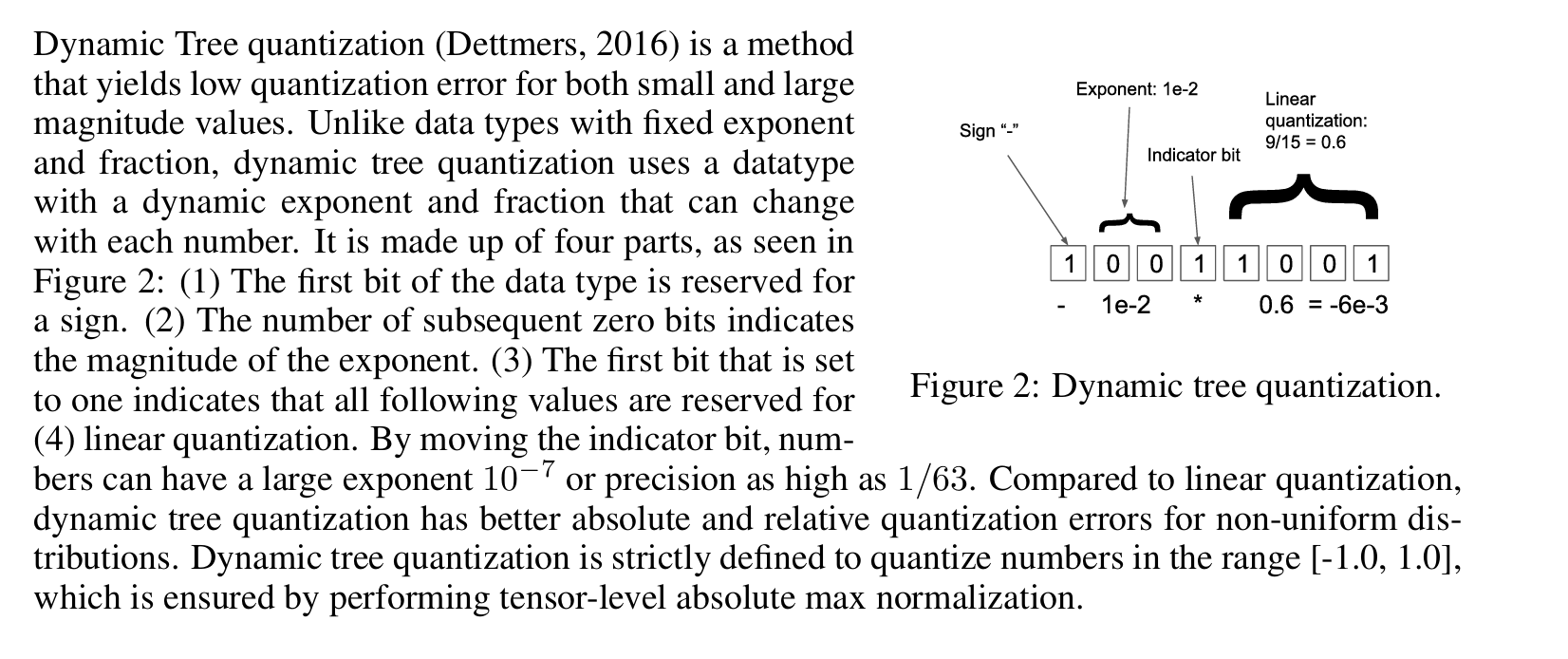
We can see that by moving the indicator bit, we will get different precision and magnitude. I guess that is why they call this non-linear quantization. For high magnitude values(less bit of exponent), the precision is higher. For low magnitude values(more bit of exponent), the precision is lower.
This is used to minimize the quantization error.
Block-wise Quantization
Let’s say we have 1B parameters and gradient values. If we apply the dynamic quantization to all of them, it is very likely that some gradient values are outliers, which means they are very large in the absolute value. Since we need to divide the largest absolute value to scale to the range between $-1.0$ and $1.0$, most of the values after this scale would be really small in absolute value and we will be not able to differentiate them. To address this problem, the authors proposed to divide the model parameters into blocks and apply the dynamic quantization to each block independently.
Another benefit of this is that GPU is highly parallalized, by apply the dynamic quantization to each block independently, they will be able to be processed in parallel. This helps address the second challenge, compuation efficiency.
Talk is cheap, show me the code
OK, we have talked a lot about the theory of the 8-bit optimizer[3]. Now let’s see how it works in practice. We can find the code at bitsandbytes repo.
State value initialization
In their Pytorch code, the initial values of the optimizer states are of type torch.uint8, shown here. This make the 8-bit optimizer states.
8-bit Quantization Candidates
This is implemented in the create_dynamic_map function. It is very similar to the theory of the Dynamic Quantization.
For each precision, the linear quantization part values are obtained linearly between $0.1$ and $1.0$ as shown in this line. Others are straight forward and I will not go into details.
Block-wise Quantization
This is very interesting because they created a special CUDA kernel for this. It is a great read to see how CUDA can help parallelize this whole process among all blocks. It is implemented in the kOptimizerStatic8bit2StateBlockwise kernel. This is the Adam[1] and AdamW[2] implementation.
quantiles1 is the 8-bit quantization candidates for the first moment of the gradient. quantiles2 is the 8-bit quantization candidates for the second moment of the gradient.
absmax1 and absmax2 are the largest absolute value of the first and second moment of the gradient for each block.
Each block will be processed by 1 thread of GPU. And that is why this is highly efficient. A few intersting points I will list here,
- Each thread will load its own quantization candidates
- Each block of the gradient values and state values are loaded into the shared memory together, shown here. Shared memory is much faster than global memory.
- Each thread de-quantizes its own state values, shown here
- Each thread updates its own state value, shown here
- Parameter values are loaded into the shared memory in parallel for each block, shown here
- Each thread will update its own parameter values with the updated state values, shown here
- The updated parameter values are stored back to the global memory, shown here. This is also done in parallel.
- The updated state values are quantized, shown here
- Finally, the quantized state values are stored back to the global memory, shown here
As an exercise, I followed the code and make it more readable. You can check it out at my cuda101.
References
[1]: @misc{kingma2017adammethodstochasticoptimization, title={Adam: A Method for Stochastic Optimization}, author={Diederik P. Kingma and Jimmy Ba}, year={2017}, eprint={1412.6980}, archivePrefix={arXiv}, primaryClass={cs.LG}, url={https://arxiv.org/abs/1412.6980}, }
[2]: @misc{loshchilov2019decoupledweightdecayregularization, title={Decoupled Weight Decay Regularization}, author={Ilya Loshchilov and Frank Hutter}, year={2019}, eprint={1711.05101}, archivePrefix={arXiv}, primaryClass={cs.LG}, url={https://arxiv.org/abs/1711.05101}, }
[3]: @misc{dettmers20228bitoptimizersblockwisequantization, title={8-bit Optimizers via Block-wise Quantization}, author={Tim Dettmers and Mike Lewis and Sam Shleifer and Luke Zettlemoyer}, year={2022}, eprint={2110.02861}, archivePrefix={arXiv}, primaryClass={cs.LG}, url={https://arxiv.org/abs/2110.02861}, }